LODA: Lightweight on-line detector of anomalies

The lightweight on-line detector of anomalies (LODA) is an outlier detection method proposed by Tomáš Pevný in 2015 article Loda: Lightweight on-line detector of anomalies 1.

LODA is a simple yet very sophisticated ensemble of weak estimators which results in a fast and robust anomaly detection model. The most significant advantages of this model are its simplicity, speed, ability to explain the cause of an anomaly, option for on-line training, and robustness to missing values.

Without going into too many technical details, the “hearth” of LODA consists of one-dimensional histograms constructed on sparse random projections. Random sparse projects allow LODA to use simple one-dimensional histograms, thus processing large datasets in relatively small time complexity. On top of that, with smart usage of their sparsity, it’s possible not only to evaluate samples with missing features but also to use them in the training process. Because histograms are one of the simplest density estimators available, they have low construction/evaluation time complexity. Anomaly score is a negative average log probability estimated from histogram on projections. Also, it has a higher time complexity than scoring samples because we need to evaluate every feature separately.

>>> import numpy as np
>>> from anlearn.loda import LODA

>>> X = np.array([[0, 0], [0.1, -0.2], [0.3, 0.2], [0.2, 0.2], [-5, -5], [0.6, 0.7]])

>>> loda = LODA(n_estimators=10, bins=10, random_state=42)
>>> loda.fit(X)
LODA(bins=10, n_estimators=10, random_state=42)
>>> loda.predict(X)
array([ 1,  1,  1,  1, -1,  1])

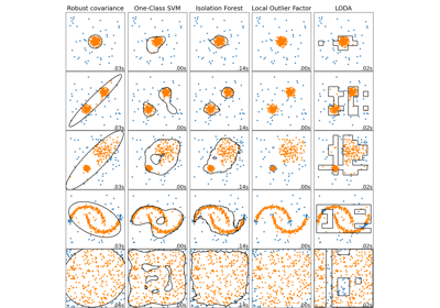
Bellow, you can see a comparison of LODA and outlier detection algorithms included in scikit-learn (Comparison of scikit-learn anomaly detection methods and LODA).

Comparison of scikit-learn anomaly detection methods and LODA

LODA parameters

LODA is a quite simple outlier detection model. Our implementation so far has only three primary parameters: n_estimators, bins, and random_seed.

• n_estimators: number of projections and histograms.

• bins: number of bins for each histogram.

• random_state: random state for stochastic parts.

• q: quantile for eveluating “anomalous” points during predict method. For detecting the “outliers” in predict method, we use the threshold evaluated from anomaly scores on training samples. For this purpose, we compute q quantile from training samples. For anomaly detection, we use the supposed percentage of abnormal points, for novelty detection 0.

See API docs for more details (anlearn.loda.LODA).

Projections and histograms

Random projections

As mentioned before, the “hearth” of LODA consists of random sparse projections and one-dimensional histograms.

Projections are sparse vectors with \(\sqrt{d}\) non-zero features (\(d\) is number of dimensions of input data). Non-zero values are generated from \(N(0; 1)\). This choice allows approximating the quantity of \(L_2\) distances between points from input space in projected space 1. Simply, we could take this as looking at the data from different angles. Sparsity also allows LODA to train and evaluate on data with missing values.

>>> loda.projections_
array([[-1.01283112,  0.        ],
       [ 0.        ,  0.31424733],
       [ 0.        , -0.90802408],
       [-1.4123037 ,  0.        ],
       [ 1.46564877,  0.        ],
       [-0.2257763 ,  0.        ],
       [ 0.        ,  0.0675282 ],
       [-1.42474819,  0.        ],
       [-0.54438272,  0.        ],
       [ 0.        ,  0.11092259]])

Right now, the number of projections is set on LODA initialization (n_estimators parameter) and initialized at the start of model fitting. In the future, we plan to implement an automatic selection for the number of projections.

See LODA: projections & histograms for full example.

LODA: projections & histograms

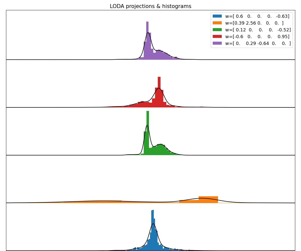
Histograms

Histograms are the second essential part of the LODA model. In our implementation, we’re using equi-width histograms. It’s more or less for practical reasons. In the LODA article experiments, we could see that this type of histograms outperformed others (section 3.3 Histogram and 4.Experiments 1). On top of that, it’s straightforward to implement and fast. In future releases, we plan to introduce more flexibility in histograms (different types, online learning, etc.).

anlearn.loda.Histogram is implemented as a scikit-learn BaseEstimator (it shares similarities with scipy.stats.rv_histogram). For detecting bin width and intervals, we’re using numpy.histogram function.

>>> loda.hists_
[Histogram(bins=10),
Histogram(bins=10),
Histogram(bins=10),
Histogram(bins=10),
Histogram(bins=10),
Histogram(bins=10),
Histogram(bins=10),
Histogram(bins=10),
Histogram(bins=10),
Histogram(bins=10)]

Explaining the cause of an anomaly

The knowledge that an example is anomalous just the first part of the whole anomaly detection pipeline. Without investigating further, I would consider this information almost useless. Lucky for us, LODA has a built-in way to get a little bit more information about why a particular example is viewed as an anomaly. With the smart usage of sparse projections, we could compute a one-tailed two-sample t-test between probabilities from histograms on projections with and without aspecific features. Casually speaking, if histograms using a particular feature have statistically higher anomaly scores than ones without it, we should have a closer look at it. Also, it has a higher time complexity than scoring samples because we need to evaluate every feature separately.

Of course, we should not consider this to be the ground truth for explaining the cause of an anomaly. That is a complicated process requiring more analysis with in-depth knowledge of data. LODA gives us only a good starting point to lead our investigation. If you want to see a full mathematical explanation read section 3.3 Explaining the cause of an anomaly 1 in the original article.

>>> loda.score_features(X)
array([[ 3.57203657, -3.57203657],
       [ 1.15114953, -1.15114953],
       [ 1.8592136 , -1.8592136 ],
       [ 1.8592136 , -1.8592136 ],
       [ 2.29212856, -2.29212856],
       [-2.23606174,  2.23606174]])

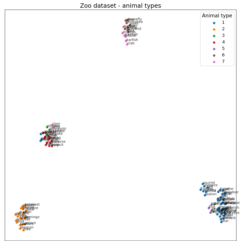
To show this feature of LODA, we created a simple example using the Zoo dataset from the UCI Machine Learning Repository 3 (LODA: Explaining the cause of an anomaly on Zoo dataset). It contains different animal species and a summary of their characteristics (hair, feathers, eggs, milk, airborne, aquatic, etc.). We have chosen it because it’s small, simple, and features are easily understandable (cat has for legs :) …) First of all, we transform this dataset using UMAP (umap.UMAP) 2 to show in two dimensions.

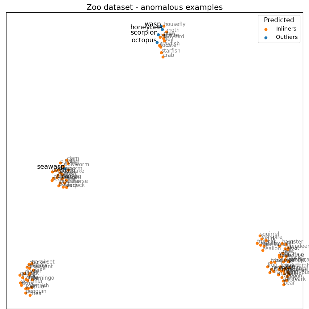
Once we get anomaly scores and importance of each feature, we could investigate further. We’ll choose the five most anomalous animals. For example, we’ll take a closer look at honeybee. It has a quite high score, and the most significant features are venomous (1.91), hair (1.55), breathes (1.28), and domestic (0.97). If we consider the composition of our dataset, there are no other venomous animals that are domestic, so it does seem right. We could find explanations like this for every other animal in the top five. Octopus has eight legs; sea wasp does have almost none of the features in the dataset, etc. So could we tell that these are the real reasons why these animals are unusual? Yes and no. Yes, this is why LODA sees them as anomalies considering our data, but without a review from a domain expert, we must be careful about such a statement. Also, consider the fact that this dataset is small, oversimplified, with just a limited number of features.

honeybee score: -4.576
        venomous 1 (1.91)
        hair 1 (1.55)
        breathes 1 (1.28)
        domestic 1 (0.97)
octopus score: -5.763
        backbone 0 (3.06)
        legs 8 (1.79)
        feathers 0 (0.96)
        toothed 0 (0.80)
scorpion score: -5.007
        legs 8 (2.18)
        toothed 0 (1.23)
        domestic 0 (1.16)
        feathers 0 (0.82)
seawasp score: -4.898
        backbone 0 (1.78)
        milk 0 (1.06)
        toothed 0 (1.05)
        feathers 0 (0.80)
wasp score: -4.579
        feathers 0 (1.99)
        fins 0 (1.43)
        catsize 0 (1.41)
        breathes 1 (1.16)

To sum it up. LODA has a really powerful tool to explain the cause of an anomaly. It is more resource consuming than scoring samples. We should take a closer look at anomalies if we want to tell the real reason.

Using LODA on large datasets

In previous sections, we have seen that LODA is fully capable of getting similar results to more complex anomaly detection methods. Now we could take full advantage of LODA’s low time and space complexity and use it on some more massive datasets.

We’ll use Credit Card Fraud Detection dataset from the Machine Learning Group of Université Libre de Bruxelles 4 (it’s available on Kaggle 5). This dataset consists of credit card transactions with 492 frauds out of 284,807 transactions. Features are a byproduct of PCA transformation without any additional information due to confidentiality issues (LODA: large data - Credit Card Fraud Detection dataset).

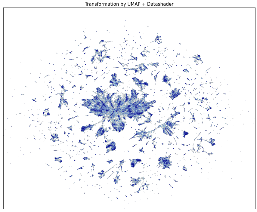
First of all, we’ll visualize the entire dataset in low dimensional space to get an overview. We’ll transform data using UMAP 2 and then plot results.

At first sight at this visualization, we could see some apparent clusters. Some of them even including a lot of fraud transactions. But this could be misleading due to significant overplotting. We’ll try to solve this issue by using a more meaningful projection created by Datashader 6.

Once we have some clues about how the dataset looks, let’s try to detect some fraud transactions. Because of its size, we’ll use only LODA and isolation forest as anomaly detection methods. For comparing them, we’ll use the area under the ROC curve.

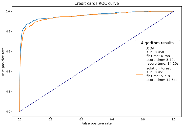
As we can see, both methods performed very well (with the LODA slightly better). The low time complexity kicks in once we look at the training/predicting time for both detectors. It took LODA only 1/4 of the isolation forest’s time to score 284,807 samples. It does not seem like such a big difference, but once we go up to millions of transactions, it could be a game-changer.

To finalize this section, let’s make another plot using Datashader and anomaly scores from LODA.

References

1(1,2,3,4)

Pevný, T. Loda: Lightweight on-line detector of anomalies. Mach Learn 102, 275–304 (2016). <https://doi.org/10.1007/s10994-015-5521-0>

2(1,2)

McInnes, L., Healy, J., Saul, N., & Grossberger, L. (2018). UMAP: Uniform Manifold Approximation and Projection The Journal of Open Source Software, 3(29), 861. <https://github.com/lmcinnes/umap/>

3

Dua, D. and Graff, C. (2019). UCI Machine Learning Repository [http://archive.ics.uci.edu/ml]. Irvine, CA: University of California, School of Information and Computer Science. <https://archive.ics.uci.edu/ml/datasets/Zoo>

4

Machine Learning Group of Université Libre de Bruxelles <http://mlg.ulb.ac.be>

5

Kaggle: Credit Card Fraud Detection <https://www.kaggle.com/mlg-ulb/creditcardfraud>

6

HoloViz Datashader <https://datashader.org/>

Examples using anlearn.loda.LODA

LODA: projections & histograms

Comparison of scikit-learn anomaly detection methods and LODA

LODA: large data - Credit Card Fraud Detection dataset

LODA: Explaining the cause of an anomaly on Zoo dataset