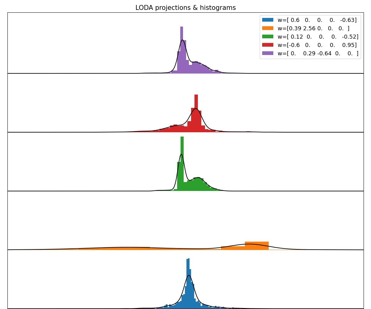
LODA: projections & histograms

# Author: Ondrej Kurák kurak@gaussalgo.com
# License: LGPLv3+
import matplotlib.pyplot as plt
import numpy as np
from scipy.stats.kde import gaussian_kde
from sklearn.datasets import make_blobs

from anlearn.loda import LODA

rng = np.random.RandomState(42)

n_inliers = 900
n_outliers = 100
n_samples = n_inliers + n_outliers

n_features = 5

data = make_blobs(
    centers=[[-2] * n_features, [2] * n_features],
    cluster_std=[1.5, 0.3],
    random_state=42,
    n_samples=n_inliers,
    n_features=n_features,
)[0]

data = np.concatenate(
    [data, rng.uniform(low=-6, high=6, size=(n_outliers, n_features))]
)

loda = LODA(n_estimators=5, bins=100, random_state=42, q=0.1)
loda.fit(data)
predicted = loda.predict(data)

plt.figure(figsize=(12, 8))
plt.subplot(111, aspect="auto")
plt.subplots_adjust(
    left=0.02, right=0.98, bottom=0.001, top=0.96, wspace=0.05, hspace=0.01
)
colors = np.array(["#377eb8", "#ff7f00"])
plt.scatter(data[:, 0], data[:, 1], s=15, color=colors[(predicted + 1) // 2])
plt.xticks(())
plt.yticks(())
plt.title("LODA test dataset anomalous points", fontsize=15)
plt.show()

w_X = loda.projections_ @ data.T

labels = [f"w={x.round(2)}" for x in loda.projections_]
n_points = 500
bounds = (np.min(w_X), np.max(w_X))

plt.figure(figsize=(12, 10))
plt.subplot(111, aspect="auto")
plt.subplots_adjust(
    left=0.02, right=0.98, bottom=0.001, top=0.96, wspace=0.05, hspace=0.01
)
xx = np.linspace(*bounds, n_points)
yticks = []
for i, tmp in enumerate(zip(w_X, labels)):
    points, label = tmp
    pdf = gaussian_kde(points)
    y = i + 0.1
    yticks.append(y)
    curve = pdf(xx)
    plt.hist(points, density=True, bottom=y, bins="auto", label=label)
    plt.plot(xx, curve + y, c="black")

plt.legend(fontsize=13)
plt.title("LODA projections & histograms", fontsize=15)
plt.xlim(bounds)
plt.yticks(())
plt.show()


# sphinx_gallery_thumbnail_number = 2