LODA: large data - Credit Card Fraud Detection dataset

In previous sections, we have seen that LODA 1 is fully capable of getting similar results to more complex anomaly detection methods. Now we could take full advantage of LODA’s low time and space complexity and use it on some more massive datasets.

We’ll use Credit Card Fraud Detection dataset from the Machine Learning Group of Université Libre de Bruxelles 4 (it’s available on Kaggle 5). This dataset consists of credit card transactions with 492 frauds out of 284,807 transactions. Features are a byproduct of PCA transformation without any additional information due to confidentiality issues.

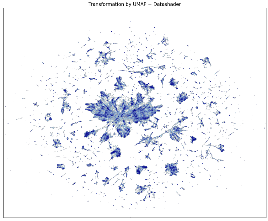
First of all, we’ll visualize the entire dataset in low dimensional space to get an overview. We’ll transform data using UMAP 2 and then plot results.

# Author: Ondrej Kurák kurak@gaussalgo.com
# License: LGPLv3+
import time

import datashader as ds
import matplotlib.pyplot as plt
import numpy as np
import pandas as pd
from colorcet import fire
from datashader import transfer_functions as tf
from sklearn.ensemble import IsolationForest
from sklearn.metrics import auc, roc_curve
from umap import UMAP

from anlearn.loda import LODA

frame = pd.read_csv("../datasets/creditcard.csv")

X = np.arcsinh(frame.values[:, 1:-1])
y = frame["Class"].values


umap = UMAP(random_state=42)

# This could take ~30 min on Intel(R) Core(TM) i5-8250U CPU @ 1.60GHz
# transformed = umap.fit_transform(X)
# with open("../datasets/transformed.npy", "wb") as out:
#     np.save(out, transformed)
transformed = np.load("../datasets/transformed.npy")


plt.figure(figsize=(12, 8))
plt.subplot(111, aspect="auto")
plt.subplots_adjust(
    left=0.02, right=0.98, bottom=0.001, top=0.96, wspace=0.05, hspace=0.01
)

for index, label in enumerate(("Normal transaction", "Fraud transaction")):
    plt.scatter(
        transformed[:, 0][y == index],
        transformed[:, 1][y == index],
        s=5,
        label=label,
        alpha=0.5,
    )

plt.legend(fontsize=13)
plt.xticks(())
plt.yticks(())

plt.title("Transformation by UMAP", fontsize=15)
plt.show()

At first sight at this visualization, we could see some apparent clusters. Some of them even including a lot of fraud transactions. But this could be misleading due to significant overplotting. We’ll try to solve this issue by using a more meaningful projection created by Datashader 6.

shader_data = pd.DataFrame(
    transformed,
    columns=["x", "y"],
)

agg = ds.Canvas(plot_width=1000, plot_height=800).points(shader_data, "x", "y")

img = tf.shade(agg, name="Transformation by UMAP + Datashader")

plt.figure(figsize=(15, 15))
plt.subplot(111, aspect="auto")
plt.subplots_adjust(top=0.96, wspace=0.05, hspace=0.01)
plt.imshow(img.to_pil())
plt.title("Transformation by UMAP + Datashader", fontsize=15)
plt.xticks(())
plt.yticks(())
plt.show()

Once we have some clues about how the dataset looks, let’s try to detect some fraud transactions. Because of its size, we’ll use only LODA and isolation forest as anomaly detection methods. For comparing them, we’ll use the area under the ROC curve.

times = {}

loda = LODA(n_estimators=100, random_state=42, bins=100)

start_time = time.monotonic()
loda.fit(X)
times["loda.fit"] = time.monotonic() - start_time

start_time = time.monotonic()
loda_scores = loda.score_samples(X)
times["loda.score_samples"] = time.monotonic() - start_time


start_time = time.monotonic()
feature_scores = loda.score_features(X)
times["loda.score_features"] = time.monotonic() - start_time

isoforest = IsolationForest(n_estimators=100, random_state=42)

start_time = time.monotonic()
isoforest.fit(X)
times["isoforest.fit"] = time.monotonic() - start_time

start_time = time.monotonic()
iso_scores = isoforest.score_samples(X)
times["isoforest.score_samples"] = time.monotonic() - start_time

loda_fpr, loda_tpr, _ = roc_curve(y, -loda_scores)
loda_auc = auc(loda_fpr, loda_tpr)

isof_fpr, isof_tpr, _ = roc_curve(y, -iso_scores)
isof_auc = auc(isof_fpr, isof_tpr)


plt.figure(figsize=(12, 8))
plt.subplot(111, aspect="auto")
plt.subplots_adjust(
    left=0.02, right=0.98, bottom=0.001, top=0.96, wspace=0.05, hspace=0.01
)

plt.plot(
    loda_fpr,
    loda_tpr,
    label=f"""LODA
 auc: {loda_auc:.3f}
 fit time: {times["loda.fit"]:.2f}s
 score time: {times["loda.score_samples"]:.2f}s,
 fscore time: {times["loda.score_features"]:.2f}s""",
)
plt.plot(
    isof_fpr,
    isof_tpr,
    label=f"""Isolation Forest
 auc: {isof_auc:.3f}
 fit time: {times["isoforest.fit"]:.2f}s
 score time: {times["isoforest.score_samples"]:.2f}s""",
)

plt.plot([0, 1], [0, 1], color="navy", linestyle="--")

plt.title("Credit cards ROC curve", fontsize=15)
plt.legend(
    title="Algorithm results", title_fontsize=15, fontsize=13, loc="center right"
)
plt.xlabel("False positive rate", fontsize=13)
plt.ylabel("True positive rate", fontsize=13)

plt.show()

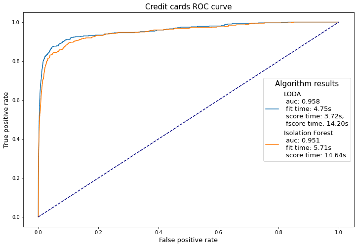
As we can see, both methods performed very well (with the LODA slightly better). The low time complexity kicks in once we look at the training/predicting time for both detectors. It took LODA only 1/4 of the isolation forest’s time to score 284,807 samples. It does not seem like such a big difference, but once we go up to millions of transactions, it could be a game-changer.

To finalize this section, let’s make another plot using Datashader and anomaly scores from LODA.

shader_data = pd.DataFrame(
    np.hstack([transformed, loda_scores[:, np.newaxis]]),
    columns=["x", "y", "anomaly_score"],
)

agg = ds.Canvas(plot_width=1000, plot_height=800).points(
    shader_data, "x", "y", ds.mean("anomaly_score")
)

img = tf.shade(
    agg, cmap=fire, name="Transformation by UMAP + Datashader (average anomaly score)"
)

img = tf.set_background(img, "black")

plt.figure(figsize=(15, 15))
plt.subplot(111, aspect="auto")
plt.subplots_adjust(
    left=0.02, right=0.98, bottom=0.001, top=0.96, wspace=0.05, hspace=0.01
)
plt.imshow(img.to_pil())
plt.title("Transformation by UMAP + Datashader (average anomaly score)", fontsize=15)
plt.xticks(())
plt.yticks(())
plt.show()

References

1

Pevný, T. Loda: Lightweight on-line detector of anomalies. Mach Learn 102, 275–304 (2016). <https://doi.org/10.1007/s10994-015-5521-0>

2

McInnes, L., Healy, J., Saul, N., & Grossberger, L. (2018). UMAP: Uniform Manifold Approximation and Projection The Journal of Open Source Software, 3(29), 861. <https://github.com/lmcinnes/umap/>

4

Machine Learning Group of Université Libre de Bruxelles <http://mlg.ulb.ac.be>

5

Kaggle: Credit Card Fraud Detection <https://www.kaggle.com/mlg-ulb/creditcardfraud>

6

HoloViz Datashader <https://datashader.org/>