Note
Click here to download the full example code
LODA: Explaining the cause of an anomaly on Zoo dataset
The knowledge that an example is anomalous just the first part of the whole anomaly detection pipeline. Without investigating further, I would consider this information almost useless. Lucky for us, LODA has a built-in way to get a little bit more information about why a particular example is viewed as an anomaly. With the smart usage of sparse projections, we could compute a one-tailed two-sample t-test between probabilities from histograms on projections with and without aspecific features. Casually speaking, if histograms using a particular feature have statistically higher anomaly scores than ones without it, we should have a closer look at it. Also, it has a higher time complexity than scoring samples because we need to evaluate every feature separately.
Of course, we should not consider this to be the ground truth for explaining the cause of an anomaly. That is a complicated process requiring more analysis with in-depth knowledge of data. LODA gives us only a good starting point to lead our investigation. If you want to see a full mathematical explanation read section 3.3 Explaining the cause of an anomaly 1 in the original article.
To show this feature of LODA, we created a simple example using the Zoo dataset from the UCI Machine Learning Repository 3.
It contains different animal species and a summary of their characteristics (hair, feathers, eggs, milk, airborne, aquatic, etc.).
We have chosen it because it’s small, simple, and features are easily understandable (cat has for legs :) …)
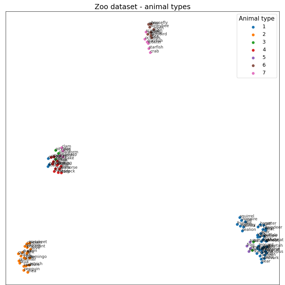
First of all, we transform this dataset using UMAP (umap.UMAP) 2 to show in two dimensions.
# Author: Ondrej Kurák kurak@gaussalgo.com
# License: LGPLv3+

import matplotlib.pyplot as plt
import numpy as np
import pandas as pd
from umap import UMAP

from anlearn.loda import LODA

frame = pd.read_csv(
    "https://raw.githubusercontent.com/sharmaroshan/Zoo-Dataset/master/zoo.csv",
)

frame.set_index("animal_name", inplace=True)

print(frame)
Out:
             hair  feathers  eggs  milk  ...  tail  domestic  catsize  class_type
animal_name                              ...
aardvark        1         0     0     1  ...     0         0        1           1
antelope        1         0     0     1  ...     1         0        1           1
bass            0         0     1     0  ...     1         0        0           4
bear            1         0     0     1  ...     0         0        1           1
boar            1         0     0     1  ...     1         0        1           1
...           ...       ...   ...   ...  ...   ...       ...      ...         ...
wallaby         1         0     0     1  ...     1         0        1           1
wasp            1         0     1     0  ...     0         0        0           6
wolf            1         0     0     1  ...     1         0        1           1
worm            0         0     1     0  ...     0         0        0           7
wren            0         1     1     0  ...     1         0        0           2

[101 rows x 17 columns]
# !cat ../datasets/zoo.names

# 1. Title: Zoo database

# 2. Source Information
#    -- Creator: Richard Forsyth
#    -- Donor: Richard S. Forsyth
#              8 Grosvenor Avenue
#              Mapperley Park
#              Nottingham NG3 5DX
#              0602-621676
#    -- Date: 5/15/1990

# 3. Past Usage:
#    -- None known other than what is shown in Forsyth's PC/BEAGLE User's Guide.

# 4. Relevant Information:
#    -- A simple database containing 17 Boolean-valued attributes.  The "type"
#       attribute appears to be the class attribute.  Here is a breakdown of
#       which animals are in which type: (I find it unusual that there are
#       2 instances of "frog" and one of "girl"!)

#       Class# Set of animals:
#       ====== ===============================================================
#            1 (41) aardvark, antelope, bear, boar, buffalo, calf,
#                   cavy, cheetah, deer, dolphin, elephant,
#                   fruitbat, giraffe, girl, goat, gorilla, hamster,
#                   hare, leopard, lion, lynx, mink, mole, mongoose,
#                   opossum, oryx, platypus, polecat, pony,
#                   porpoise, puma, pussycat, raccoon, reindeer,
#                   seal, sealion, squirrel, vampire, vole, wallaby,wolf
#            2 (20) chicken, crow, dove, duck, flamingo, gull, hawk,
#                   kiwi, lark, ostrich, parakeet, penguin, pheasant,
#                   rhea, skimmer, skua, sparrow, swan, vulture, wren
#            3 (5)  pitviper, seasnake, slowworm, tortoise, tuatara
#            4 (13) bass, carp, catfish, chub, dogfish, haddock,
#                   herring, pike, piranha, seahorse, sole, stingray, tuna
#            5 (4)  frog, frog, newt, toad
#            6 (8)  flea, gnat, honeybee, housefly, ladybird, moth, termite, wasp
#            7 (10) clam, crab, crayfish, lobster, octopus,
#                   scorpion, seawasp, slug, starfish, worm

# 5. Number of Instances: 101

# 6. Number of Attributes: 18 (animal_name, 15 Boolean attributes, 2 numerics)

# 7. Attribute Information: (name of attribute and type of value domain)
#    1. animal_name:      Unique for each instance
#    2. hair                Boolean
#    3. feathers            Boolean
#    4. eggs                Boolean
#    5. milk                Boolean
#    6. airborne            Boolean
#    7. aquatic             Boolean
#    8. predator            Boolean
#    9. toothed             Boolean
#   10. backbone            Boolean
#   11. breathes            Boolean
#   12. venomous            Boolean
#   13. fins                Boolean
#   14. legs                Numeric (set of values: {0,2,4,5,6,8})
#   15. tail                Boolean
#   16. domestic            Boolean
#   17. catsize             Boolean
#   18. class_type          Numeric (integer values in range [1,7])

# 8. Missing Attribute Values: None

# 9. Class Distribution: Given above
Data visualization
X = frame.values[:, :-1]

# Prepare data for visualization using UMAP
umap = UMAP(n_neighbors=15, min_dist=0.9, random_state=42)
transformed = umap.fit_transform(X)

plt.figure(figsize=(10, 10))
plt.subplot(111, aspect="auto")
plt.subplots_adjust(
    left=0.02, right=0.98, bottom=0.001, top=0.96, wspace=0.05, hspace=0.01
)


for type in np.unique(frame["class_type"]):
    selected = transformed[frame["class_type"] == type]
    plt.scatter(selected[:, 0], selected[:, 1], label=type)

for name, x, y in zip(frame.index, transformed[:, 0], transformed[:, 1]):
    plt.annotate(name, (x, y), alpha=0.8, fontsize=10)

plt.title("Zoo dataset - animal types", fontsize=18)
plt.xticks(())
plt.yticks(())
plt.legend(title="Animal type", title_fontsize=15, fontsize=13)
plt.show()
Explaining the cause of an anomaly
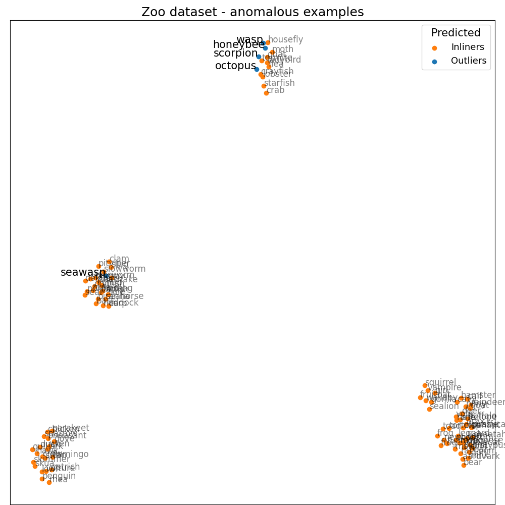
Once we get anomaly scores and importance of each feature, we could investigate further. We’ll choose the five most anomalous animals. For example, we’ll take a closer look at honeybee. It has a quite high score, and the most significant features are venomous (1.91), hair (1.55), breathes (1.28), and domestic (0.97). If we consider the composition of our dataset, there are no other venomous animals that are domestic, so it does seem right. We could find explanations like this for every other animal in the top five. Octopus has eight legs; sea wasp does have almost none of the features in the dataset, etc. So could we tell that these are the real reasons why these animals are unusual? Yes and no. Yes, this is why LODA sees them as anomalies considering our data, but without a review from a domain expert, we must be careful about such a statement. Also, consider the fact that this dataset is small, oversimplified, with just a limited number of features.
loda = LODA(n_estimators=100, bins=100, random_state=42)
loda.fit(X)

scores = loda.score_samples(X)
predicted = loda.predict(X)


plt.figure(figsize=(10, 10))
plt.subplot(111, aspect="auto")
plt.subplots_adjust(
    left=0.02, right=0.98, bottom=0.001, top=0.96, wspace=0.05, hspace=0.01
)

X_n = transformed[predicted == 1]
X_a = transformed[predicted == -1]

plt.scatter(X_n[:, 0], X_n[:, 1], color="tab:orange", label="Inliners")
plt.scatter(X_a[:, 0], X_a[:, 1], color="tab:blue", label="Outliers")

for name, x, y in zip(frame.index[predicted == 1], X_n[:, 0], X_n[:, 1]):
    plt.annotate(name, (x, y), alpha=0.5, fontsize=12)

for name, x, y in zip(frame.index[predicted == -1], X_a[:, 0], X_a[:, 1]):
    plt.annotate(name, (x, y), fontsize=15, ha="right")

plt.title("Zoo dataset - anomalous examples", fontsize=18)
plt.legend(title="Predicted", title_fontsize=15, fontsize=13)
plt.xticks(())
plt.yticks(())
plt.show()

feature_scores = loda.score_features(X)

for animal, score, feature_score in zip(
    frame[predicted == -1].itertuples(),
    scores[predicted == -1],
    feature_scores[predicted == -1],
):
    name = animal[0]
    srt = np.argsort(feature_score)[::-1]

    print(f"{name} score: {score:.3f}")

    for feature, value, importance in zip(
        frame.columns[srt][:4], np.array(animal[1:])[srt], feature_score[srt]
    ):
        print(f"\t{feature} {value} ({importance:.2f})")
Out:
honeybee score: -4.576
        venomous 1 (1.91)
        hair 1 (1.55)
        breathes 1 (1.28)
        domestic 1 (0.97)
octopus score: -5.763
        backbone 0 (3.06)
        legs 8 (1.79)
        feathers 0 (0.96)
        toothed 0 (0.80)
scorpion score: -5.007
        legs 8 (2.18)
        toothed 0 (1.23)
        domestic 0 (1.16)
        feathers 0 (0.82)
seawasp score: -4.898
        backbone 0 (1.78)
        milk 0 (1.06)
        toothed 0 (1.05)
        feathers 0 (0.80)
wasp score: -4.579
        feathers 0 (1.99)
        fins 0 (1.43)
        catsize 0 (1.41)
        breathes 1 (1.16)
Summary
To sum it up. LODA has a really powerful tool to explain the cause of an anomaly. It is more resource consuming than scoring samples. We should take a closer look at anomalies if we want to tell the real reason.
References
- 1
Pevný, T. Loda: Lightweight on-line detector of anomalies. Mach Learn 102, 275–304 (2016). <https://doi.org/10.1007/s10994-015-5521-0>
- 2
McInnes, L., Healy, J., Saul, N., & Grossberger, L. (2018). UMAP: Uniform Manifold Approximation and Projection The Journal of Open Source Software, 3(29), 861. <https://github.com/lmcinnes/umap/>
- 3
Dua, D. and Graff, C. (2019). UCI Machine Learning Repository [http://archive.ics.uci.edu/ml]. Irvine, CA: University of California, School of Information and Computer Science. <https://archive.ics.uci.edu/ml/datasets/Zoo>
Total running time of the script: ( 0 minutes 6.799 seconds)